Optimizing CPU & Memory Interaction: Matrix Multiplication

Same algo, different memory access patterns, what could go wrong (or right)!

Introduction

Matrix multiplication is a classic example for demonstrating how memory access patterns significantly impact an algorithm’s runtime. The O(N^3) algorithm remains unchanged but by optimizing the way memory accessed, we can improve the runtime by as much as 40x.

Straightforward algorithm

We’ll be focusing on NxN (square) matrices where N is assumed to be very large.

Matrix multiplication involves taking two matrices A and B and combining them into a new matrix C.

matrix multiplication diagram credits wikipedia

For each element in C, we take the dot product of the associated row in A with the associated column in B. The mathematical definition from wikipedia is definitely clearer and more precise:

matrix multiplication formula credits wikipedia

This definition also lends itself to the following straightforward algorithm [1]:

#define N 2
typedef double matrix[N][N];

void multiply(matrix A, matrix B, matrix C, int n) {
    for (int i = 0; i < n; i++) {
        for (int j = 0; j < n; j++) {
            double res = 0.0;
            for (int k = 0; k < n; k++) {
                res += A[i][k] * B[k][j];
            }
            C[i][j] = res;
        }
    }
}

int main() {
    matrix A = { { 1, 2}, { 3, 4} };
    matrix B = { { 5, 6}, { 7, 8} };
    matrix C = { 0 };
    multiply(A, B, C, N);
    // C: [ 19.0  22.0
    //      43.0  50.0 ]
    return 0;
}

A couple of points worth pointing out from the above code snippet:

Its complexity is O(N^3) where N is the length/width of the matrix. For each entry in C, we do N amount of work, there are N^2 entries, thus N^3.
Every entry per source element (A & B) is read N times

The goal of this post is to detail how the straightforward approach can be optimized with regards to memory accesses. Before going any further, we’ll need to introduce caching in computer systems, plus some key terms and definitions:

Caches & Locality

A basic computer system consists of the CPU and a memory system for data storage. Transferring data back and forth from memory is quite slow from the CPU’s perspective. Therefore, in practice, a cache is added in between the CPU and memory to speed up access and bridge the processor-memory gap.

Note, in this discussion, I’ll treat the cache as a unified component but if you dig further in [1], the cache is in fact composed of multiple caches (L1, L2, L3) each organized hierarchically with the higher caches (the ones closer to the CPU) holding a smaller subset of the data compared to the lower ones.

The cache’s function is twofold: keep frequently accessed data close to the CPU and keep neighbouring data close by. This strategy leverages the concept of locality.

Programs usually exhibit two kinds of locality that contribute to the effectiveness of caching:

temporal locality: once a program references a memory location, it’s likely to reference it again multiple times in the near future [1].
spatial locality: once a program references references a memory location, it’s likekly to reference nearby locations in the near future [1].

Thus, caching the contents of a memory address plus the adjacent data into a singular block that’s stored in a cache line advances both temporal and spatial locality.

Caches, Reads and Writes

With caches in the picture, reads and writes carried out by the CPU become a bit more complicated.

When the CPU performs a read for a word (the data unit referenced by an address), the word’s associated block is first checked in the the cache. If the block is present, we get a cache hit. However, if absent, we get a cache miss: its block has to be fetched from memory, then the address’s contents loaded into a register in the CPU.

As detailed in [1], writes are a bit more complex. There are two cases:

write hit: the address being written to is already in the cache as a block. When writing to it, there are two approaches:
- write-through: upon writing to the cached block, also update its underlying block in the memory. Advantages: You can evict a cache line without having to write it to memory. Also, in a multi-core setup, it guarantess consistency trivially. Disadvantage: every write results in a block transfer back to memory; this increases traffic/decreases relative performance.
- write-back: defer updating the underlying block in memory until necessary (such as when evicting the block from the cache). Meanwhile, the block in memory remains stale. Advantage: decreases traffic by exploiting locality (we might write to the same location soon or to nearby locations). Disadvantage: Implementation is more complex - in a multi-core setup, we now require a cache coherency protocol to maintain consistency [3]. Additionally, some evictions will result in writes to memory [3].
write miss: the address being written to isn’t cached. We have two options:
- write allocate: Also called fetch-on-write. As its alternate name suggests, it involves fetching the associated block from memory into cache, then treating it as a write hit (use either write-through or write-back approaches). Advantages: exploits locality especially if paired with the write-back approach. Disadvantage: every write-miss results in a block transfer into the cache.
- no write allocate: on a write-miss, bypass the cache and write the data unit directly to memory. The cached block has to be invalidated such that if read soon after the write, it should result in a cache miss. It’s advantageous in situations where we’re writing to an object that won’t be read any time soon hence we can avoid allocating cache lines that won’t get used (cache pollution).

Since write-back and write-allocate complement each other well with regards to locality, they are often paired.

Exploiting locality

Given that caches leverage locality, for optimal performance, we need to exploit both temporal & spatial locality when writing our programs. Let’s start with a simple example, summing up all the values in a two dimensional array:

double get_sum(double a[M][N]){
  double res = 0.0;
  for (double i = 0; i < M; i++){
      for (double j = 0; j < N; j++){
          res += a[i][j];
        }
    }
  return res; 
}

This seemingly simple snippet takes advantage of both temporal and spatial locality. The 2-D array consists of M rows each containing N columns (i.e. N doubles). In C, such arrays are laid out in memory in a row-major order. Therefore, when summing up the elements in the above snippet, the inner-loop iterates through the first row, then the second row and so forth [1]. The local variable res should be cached in the CPU register by the compiler therefore making iterative writes to it fast (temporal locality). Upon a cache miss, chunks of the array are loaded into memory block by block. Thus, the next read is a cache hit enabling the program to take advantage of spatial locality.

Now, suppose we interchange the i and j loops as follows:

double get_sum(double a[M][N]){
  double res = 0.0;
  for (double j = 0; j < N; j++){
    for (double i = 0; i < M; i++){
          res += a[i][j];
        }
    }
  return res; 
}

The program traverses the 2-D array by going down the first column, then the second and so on.

row-major traversal vs column-major traversal

It’s still the same from a correctness perspective (though I’m not quite sure addition of doubles is commutative, but let’s assume). And it still does the same amount of work from a theoretic/complexity perspective (O(MN)), particularly if we treat referencing random memory as a constant operation. However, its “actual” performance is quite poor compared to the prior row-by-row version. Given how 2-D arrays are laid out, it fails to take advantage of spatial locality. In fact, if N is set to the size of the cache, each inner-loop addition requires a fetch from a lower level and might even evict previous rows that we’ll need to access again when summing up the next column. All these make the performance gap quite evident.

When carrying out a benchmark to demonstrate the performance gap between summing row-by-row vs column-by-column, I get the following results:

sum by row vs by col

Summing row-by-row is 28.8% faster. In this case, each row has 512 doubles and there are 1024 rows. As an aside, I ported the prior C code snippet to Rust and used criterion for the benchmarking just to get a handle of how microbenchmarks can be carried out in Rust.

Regardless, in both cases, we see what’s referred to as a stride pattern. The row-by-row version exhibits a stride-1 pattern - the best-case for spatial locality. The column-by-column version exhibits a stride-N pattern, the larger N is the more spatial locality decreases.

Key Takeaways so Far

Let’s pause a bit and take stock of the ‘best practices’ highlighted so far (all these are referenced from [1]):

when iterating, take into account the stride and try to reduce it as much as possible so as to exploit spatial locality. Stride-1/sequential access is optimal given that contiguous data in memory is cached in blocks.
use/re-use a data-object as much as possible to maximize temporal locality
when optimizing for writes, for simplicity’s sake, assume the caches are write-back write-allocate. These already tends to be the case in modern computer systems. For example in my laptop (purchased in 2020), the L1 d-cache,L2 and L3 caches are write-back and presumably write-allocate. In linux, you can use the dmidecode tool to check your cache info(dmidecode -t cache)
for nested loops, pay attention to the innermost loop since it’s where the bulk of the work is done.

Now, back to matrix multiplication:

AB Routines for Matrix Multiplication

Recall we started with the following straightforward matrix multiplication routine:

int i, j, k;
for (i = 0; i < N; i++) {
    for (j = 0; j < N; j++) {
        double r = 0.0;
        for (k = 0; k < N; k++) {
            r += A[i][k] * B[k][j];
        }
        C[i][j] = r;
    }
}

The outermost loop increments i, then the middle loop increments j, then the innermost loop increments k. We shall refer to this as the ijk version.

Let’s focus on the work being done in the innermost-loop:

r += A[i][k] * B[k][j];

Given that k is incrementing in the innermost loop while i and j remain constant, the traversal of A is row-wise with a stride of 1 while the traversal of B is column-wise with a stride of n (n is assumed to be very large thus negating any instance of spatial locality).

AB traversals

Additionally, each iteration involves 2 loads (reads from A and B), and zero stores. Suppose a cache line holds 64 bytes and a double is 8 bytes. With the row-wise traversal of A, we’ll get a cache miss when loading the 0th value in a block and cache hits on the next 7 values. Therefore each iteration will involve 0.125 misses when referencing A. With the column-wise traversal of B, each reference per iteration will result in a cache miss. We ignore the store involving C since it’s done outside and majority of the work/time spent will be inside the loop. In total, there will be 1.125 misses per iteration.

Now that we have a bit of experience interchanging for-loops, we could switch i-j to j-i as follows. This will be the jik version:

int i, j, k;
for (j = 0; j < N; j++) {
    for (i = 0; i < N; i++) {
        double r = 0.0;
        for (k = 0; k < N; k++) {
            r += A[i][k] * B[k][j];
        }
        C[i][j] = r;
    }
}

As we’ll see in the benchmark results section, ijk and jik have essentially the same performance due to having the same memory access pattern (1.125 misses per innermost iteration) in the innermost for-loop. Thus, they both fall under the same equivalence class of AB.

Can we do better? Yes, definitely:

BC Routines for Matrix Multiplication

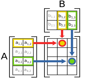
Let’s start with the following diagram:

Loop directions for i,j,k

Observe that if we make the for-loop for j the innermost one, we’ll get a row-wise traversal of matrix B and C which will be of stride-1, thus maximizing spatial locality.

Translating this into code, we get:

int i, j, k;
for (k = 0; k < N; k++) {
    for (i = 0; i < N; i++) {
        for (j = 0; j < N; j++) {
          C[i][j] += A[i][k] * B[k][j];
        }
    }
}

A[i][k] remains constant in the innermost loop therefore we can place it in a temporary variable and the compiler will cache it in one of the CPU registers:

// kij
int i, j, k;
for (k = 0; k < N; k++) {
    for (i = 0; i < N; i++) {
        double r = A[i][k];
        for (j = 0; j < N; j++) {
          C[i][j] += r * B[k][j];
        }
    }
}

As is the case for the AB class, we can permute the k and i for-loops to get kij and ikj versions:

// ikj
int i, j, k;
for (i = 0; i < N; i++) {
    for (k = 0; k < N; k++) {
        double r = A[i][k];
        for (j = 0; j < N; j++) {
            C[i][j] += r * B[k][j];
        }
    }
}

Both versions should have the same performance since they entail the same memory access patterns:

BC traversals

Let’s analyze the work getting done per each iteration (of the innermost for-loop):

C[i][j] += r * B[k][j];

Suppose the cache is write-back, write-allocate and a cache line holds 64 bytes. Both B and C are being traversed row-wise with a stride of 1. We’ve got two loads: one for B[k][j], and one for C[i][j], which has to be loaded before getting updated. This update does involve a subsequent store operation. The store operation will not result in a write miss due to the preceding load. The load involving A is ignored since it’s carried out outside the loop. There will be a cache miss every 0th load and the next 7 values will be straight cache hits. Therefore there will be 0.25 (0.125 + 0.125) misses per iteration vs the 1.125 for AB routines.

Despite BC routines carrying out more memory accesses per iteration compared to AB routines (2 loads and 1 store vs 2 loads only), they perform better courtesy of less cache misses per iteration. The store doesn’t end up hurting performance as much since under a write-back system, the writes can go directly to the cache and only during eviction does the memory get updated [4].

While we’ve seen how we can get better performance, it’s worth also seeing how we can get way worse performance.

AC Routines for Matrix Multiplication

By making the innermost for-loop be the one that increments i, we get the AC routines: jki and kji. These traverse A and C column by column:

AC traversals

Applying the same kind of analysis as for AB and BC routines, there will be 2 loads and a store per iteration and 2 cache misses per iteration due to the stride of n.

For the sake of completion, here’s the code sample for jki and kji

// jki
int i, j, k;
for (j = 0; j < N; j++) {
    for (k = 0; k < N; k++) {
        double r = B[k][j];
        for (i = 0; i < N; i++) {
            C[i][j] += A[i][k] * r;
        }
    }
}

// kji
int i, j, k;
for (k = 0; k < N; k++) {
    for (j = 0; j < N; j++) {
        double r = B[k][j];
        for (i = 0; i < N; i++) {
            C[i][j] += A[i][k] * r;
        }
    }
}

Benchmark Results

So far I’ve been alluding to the great performance of BC routines without showing the actual results. So without further ado, here’s the graph comparing all the routines:

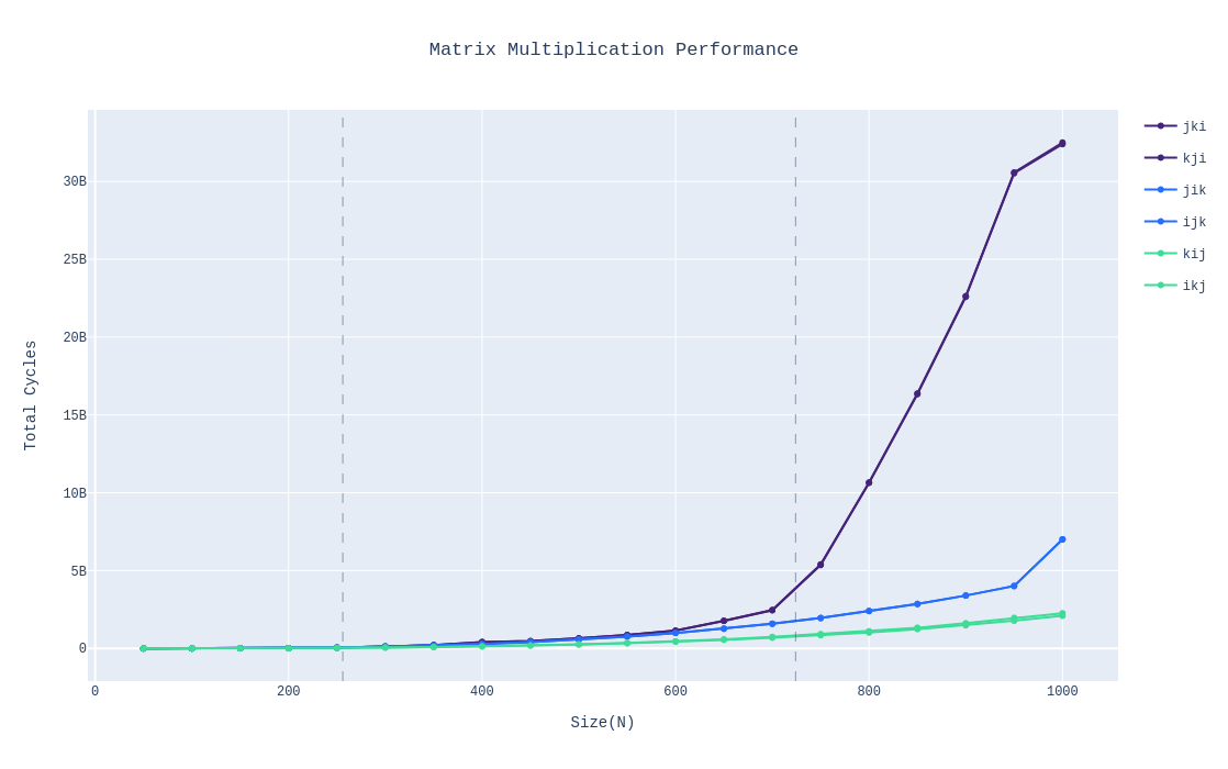
Line chart comparing total cycles for each matrix multiplication routine

Routines within the same class have essentially the same performance, seeing as their graphs are indistinguishable. The graphs’s divided into three regions, in the leftmost region, all data should fit entirely in L2; in the middle region, all the data should fit in L3; in the rightmost region, the data is larger than L3. However, I did make a mistake in the demarcation between L2 and L3, the size of L2 in the graph is larger than it should be. Nonetheless, we see that once data no longer fits in L3, the performance between the three classes starts diverging with the AC class routines getting significantly slower compared to the rest.

We’ve also got the following:

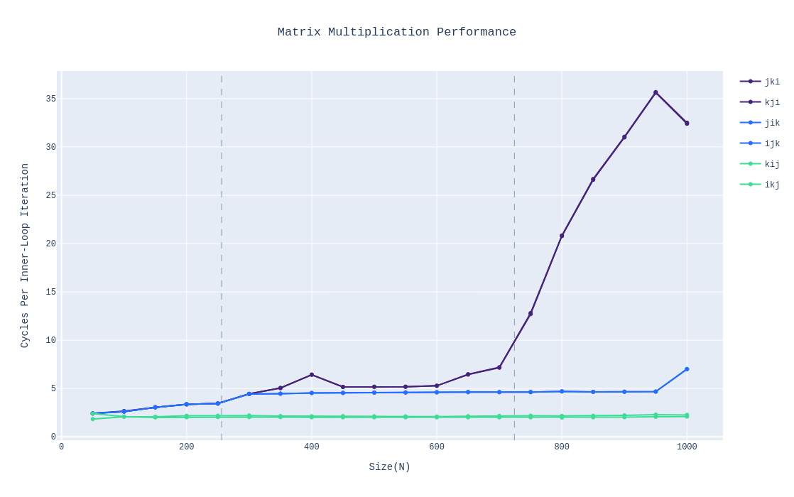
Line chart comparing cycles per inner-loop iteration for each matrix multiplication routine

In this, we measure how many cycles a single innermost loop takes, that is, one instance of the multiplication and addition. BC(kij & ikj) remains consistent throughout even as the number of elements increases. AB(ijk & jik) also remains consistent though it spends roughly twice the number of cycles as BC. However, with AC(jki and kji), once the data can no longer fit in L3, its performance degrades heavily since every iteration entail two separate memory accesses with the cache blocks not even getting re-used before they’re evicted.

Regardless, as pointed out in [1], miss rate dominates performance which demonstrates the need for factoring cache usage when designing and optimizing algorithms.